Experiment 6. COMPTON SCATTERING OF GAMMA RAYS

In the elastic scattering of a photon through angle a by a free electron initially at rest, the energy E' of the scattered photon is given in terms of the energy E of the incident photon and rest energy of the electron, mc², by

E' = E / [ 1 + E/mc²(1- cos(a)) ].

While for optical photons E is much less than mc² (=0.511 MeV) and energy changes are small, large shifts are predicted for gamma rays of energy E ~ mc². In this experiment, you will study scattering of a beam of 0.662 MeV gamma rays from a plastic target and detect the scattered radiation using a NaI scintillation detector.

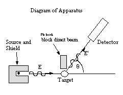
Equipment: Intense collimated beam of ¹³⁷Cs gammas, target of low Z, movable NaI scintillation detector in a table-top scattering apparatus.

Readings: Compton scattering, theory and experiment: 6.3.1-6.3.3.

Key concepts: Compton scattering; Thomson and Klein-Nishina differential scattering crosssections.

Radiation safety: The radioactive source used in this experiment, ~5 mCi of ¹³⁷Cs, is much stronger than others used in this course; take precautions to limit your exposure.

Before the laboratory. Calculate the energy of 0.662 MeV gamma rays scattered through angles of 120^o and 60^o.

6.1 Energy Calibration

Calibrate energy versus channel-number of the pulse-height analyzer for the NaI detector used. Using a weak ¹³⁷Cs source, set the amplifier gain so that the 0.662 MeV photopeak falls close to the top of PHA memory. Then use sources of other isotopes to check calibration and linearity.

6.2 Energy versus scattering angle

Measure pulse-height spectra for different scattering angles at ~10^o intervals, covering as wide a range of angles as possible. Determine the angles and their uncertainties from the geometry. These measurements may also be used for anslysis of scattering crosssections (see below) so record distances carefully and save spectra for future reference. Place lead blocks between the source and target to reduce unwanted 'background' counts.

There will be a substantial background counting rate.. To eliminate background radiation from your spectra, accumulate a spectrum in the PHA with the target in place, then subtract counts accumulated over the same length of time after removing the target. Count for a sufficent time so that the position of the photopeak can be determined to within 10-20 keV (~10-15 minutes). Difference spectra can be calculated either in a spreadsheet program or using special functions of the Tracor-Northern PHA. Save difference spectra at each angle and determine the energy of the photopeak and its uncertainty. Set up your experimental geometry carefully, and estimate the uncertainty in your measurements of the scattering angle.

It can be shown from Compton's theory that 1/E' should vary proportionally with (1- cos(a)). Plot your data in that way and determine a "best" straight line through the data either numerically or graphically. Evaluate the rest energy of the electron (and its uncertainty) from the slope of your plot. Discuss your results.

6.3 Scattering crosssection

Measure background-corrected difference spectra as in part 2, but count for a uniform live time and integrate each spectrum to determine the relative counting rate at each angle. Keep the detector at a carefully fixed distance from the target to avoid changes of solid angle (~1/r² ). Avoid counting the direct beam at small angles. Integrated counts under the difference spectra are proportional to the scattered flux. To get relative crosssections, you will need to correct the integrals for the detection efficiency, which is energy dependent.

Plot relative crosssections versus angle, as in fig. 6.14. Compute and draw the Klein-Nishina crosssection on your figure, after normalizing it to your data near 100-120^o where the crosssection is fairly constant. Discuss your results.

6.4 Absolute crosssections

The scattered flux is proportional to the total number of scattering centers (free electrons) in the beam. Determine the absolute crosssection by measuring the beam flux, solid angles and the number of electrons in the target, following procedures like those described on pages 261-265. Estimate the uncertainty in your determination by propagation of errors.

6.5 Background reduction by coincidence counting

If a plastic scintillation detector and coincidence circuit are available, then the experiment can be carried out in a different way to reduce backgrounds. Note that the scattered electron has significant kinetic energy and will produce a light pulse in a scintillator used as a target. Using the plastic scintillator as the target, accumulate pulses detected in the movable NaI detector that are coincident in time with pulses in the plastic detector.

6.6 Photofraction versus photon energy

By looking at photons scattered through different angles, you can "tune" the photon's energy. Analyse the photofractions of the difference spectra collected in part 2. Plot the photofraction versus energy and try to interpret your graph using tabulated values of the photoelectric and Compton scattering crosssections from the literature or from a URL such as http://www.csrri.iit.edu/periodic-table.html . .

Questions and considerations

a. Why is a plastic or other low-Z target preferred in this experiment? Would an Al or Pb rod work well as a target?

b. Analysis of scattering angles is simplified by using the average scattering angle. Under what assumptions will the average scattering angle equal the geometrical angle shown in the diagram above? Consider the validity of the assumptions.

c. What influence does the finite angular extents of your target and detector have on your measurements? Can you substantiate any such influences quantitatively?

d. How far would the target need to have been displaced from its ideal position to substantially affect your measurements?